Errors Are Unavoidable When Classes Overlap
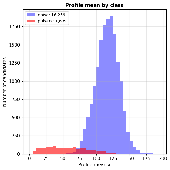
Data: 17,898 human-labeled pulsar candidates from a radio-telescope survey
- Pulsars (\(Y = 1\)): 1,639, 9.2%
- Noise (\(Y = 0\)): 16,259
Measurement \(x\): the mean of the candidate’s pulse profile
- Pulsars average 56.7, noise 116.6
Decision: pulsar or noise, from \(x\) alone
Overlap: the same \(x\) occurs in both classes
- \(x\) from 70 to 80: 145 pulsars and 250 noise
- Any rule based on \(x\) alone misclassifies some candidates
Data: HTRU2, R. J. Lyon et al., MNRAS 2016; UCI Machine Learning Repository (CC BY 4.0)
Different Thresholds Trade Misses for False Alarms
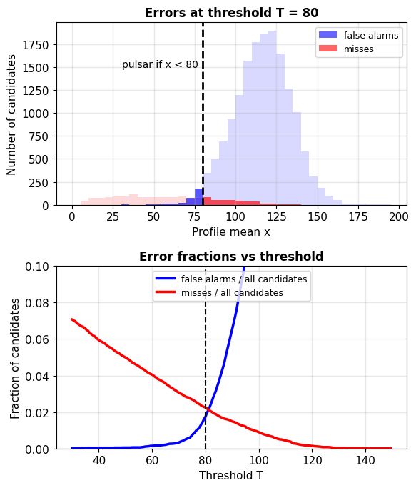
Rule: decide pulsar if \(x < T\), noise otherwise
Two errors:
- False alarm: noise decided as pulsar, \(P(Y{=}0,\ X < T)\)
- Miss: pulsar decided as noise, \(P(Y{=}1,\ X \ge T)\)
Example, \(T = 80\), counted over the 17,898 candidates:
- False alarms: 309 candidates (1.7% of all, 1.9% of noise)
- Misses: 404 candidates (2.3% of all, 25% of pulsars)
Raising \(T\): fewer misses, more false alarms
- The classes overlap: both errors are nonzero for every \(T\)
Risk Is the Expected Loss of a Decision Rule
Decision rule \(\delta(\mathbf{x})\): an action for each \(\mathbf{x}\)
- Binary: decide 1 (pulsar) or 0 (noise)
Loss \(c(y, a)\): cost of action \(a\) when the class is \(y\)
\[\mathbf{C} = \begin{bmatrix}
c_{00} & c_{01} \\
c_{10} & c_{11}
\end{bmatrix} = \begin{bmatrix}
0 & 1 \\
10 & 0
\end{bmatrix}\]
- Row: class, column: action
- \(c_{01} = 1\): one wasted telescope observation per false alarm
- \(c_{10} = 10\): a missed pulsar, valued at 10 such observations
Risk:
\[R(\delta) = \mathbb{E}[c(Y, \delta(X))] = c_{01}\,P(\text{false alarm}) + c_{10}\,P(\text{miss})\]
Example, counted over the candidates:
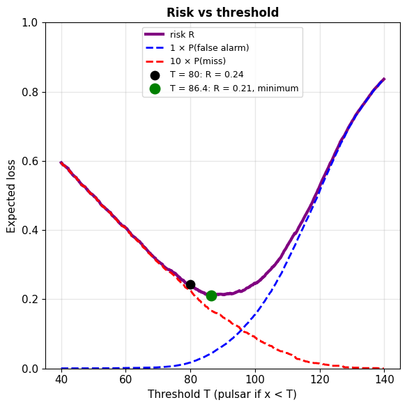
- \(T = 80\): \(R = 0.017 + 10 \times 0.023 = 0.24\)
- \(T = 86.4\): \(R = 0.21\), the smallest
Bayes rule \(\delta^*\): the rule with the smallest risk
The Bayes Rule Depends on \(\mathbf{x}\) Only Through \(P(Y \mid \mathbf{x})\)
Risk by iterated expectations:
\[R(\delta) = \mathbb{E}_X\Big[\, \mathbb{E}[c(Y, \delta(X)) \mid X] \,\Big]\]
- The inner term depends only on the action at that \(\mathbf{x}\)
- Choosing the smallest inner term at every \(\mathbf{x}\) minimizes the risk
Bayes rule:
\[\delta^*(\mathbf{x}) = \arg\min_a \sum_k c(k, a)\, P(Y=k \mid \mathbf{x})\]
Binary, with \(\pi(\mathbf{x}) = P(Y=1 \mid \mathbf{x})\):
- Expected loss of deciding noise: \(c_{10}\, \pi(\mathbf{x})\)
- Expected loss of deciding pulsar: \(c_{01}\, (1 - \pi(\mathbf{x}))\)
- Bayes rule: the smaller of the two
\(\pi(\mathbf{x}) = \mathbb{E}[Y \mid X = \mathbf{x}]\): for \(Y \in \{0,1\}\), the posterior is the MMSE predictor
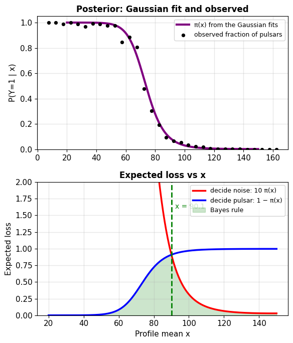
Example: a Gaussian fitted to each class, \(\mathcal{N}(116.6, 17.5^2)\) for noise and \(\mathcal{N}(56.7, 30.0^2)\) for pulsars, with \(P(Y{=}1) = 0.092\)
- Expected losses equal at \(x = 90.1\)
- Minimum-risk threshold from counting: 86.4
The MAP Rule Minimizes Risk Under 0-1 Loss
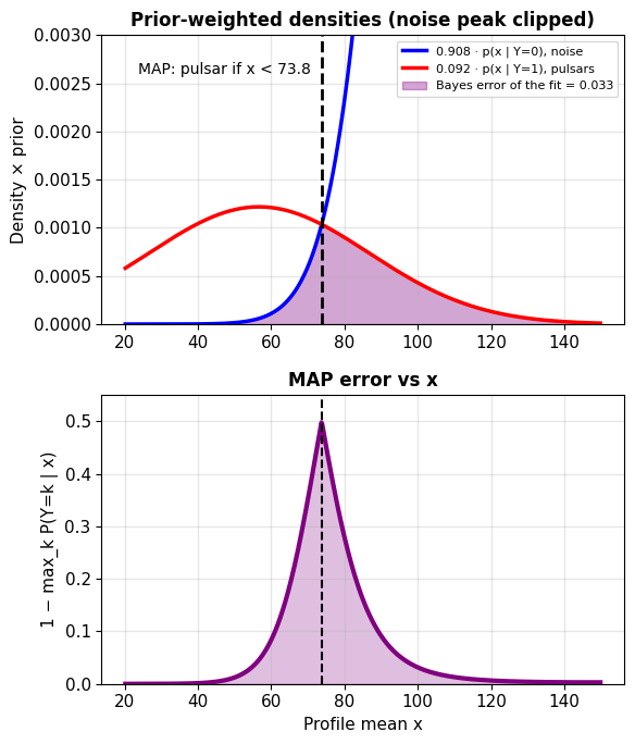
0-1 loss: every error costs 1, so the risk is the probability of error
Expected loss of deciding class \(a\): \(1 - P(Y=a \mid \mathbf{x})\)
MAP rule: the class with the largest posterior
\[\delta_{\text{MAP}}(\mathbf{x}) = \arg\max_k P(Y=k \mid \mathbf{x})\]
- Binary: decide 1 when \(\pi(\mathbf{x}) > 1/2\)
Bayes error: the error rate of the MAP rule
\[\mathbb{E}\Big[1 - \max_k P(Y=k \mid X)\Big]\]
- No rule has a lower error rate
- Counterpart of \(\mathbb{E}[\text{Var}(Y \mid X)]\), the minimum MSE
Example: decide pulsar when \(x < 73.8\), where the fitted \(\pi(x) = 1/2\)
- 3.4% of candidates misclassified
- Deciding noise for every candidate: 9.2%
- 30% of pulsars decided as noise
Bayes Threshold on \(\pi\) = \(c_{01}/(c_{01} + c_{10})\)
Decide pulsar when its expected loss is smaller:
\[c_{01}(1-\pi) < c_{10}\,\pi \quad\Longleftrightarrow\quad \pi > \frac{c_{01}}{c_{01} + c_{10}}\]
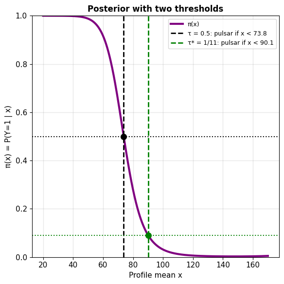
Threshold on the posterior:
\[\tau^* = \frac{c_{01}}{c_{01} + c_{10}}\]
- Equal costs: \(\tau^* = 1/2\), the MAP rule
- Costlier misses: \(\tau^* < 1/2\)
Example, \(c_{01} = 1\), \(c_{10} = 10\): \(\tau^* = 1/11 = 0.091\)
| Rule | Pulsar if | Misses | False alarms |
|---|---|---|---|
| MAP, \(\tau = 0.5\) | \(x < 73.8\) | 30% of pulsars | 0.6% of noise |
| Costs, \(\tau^* = 0.091\) | \(x < 90.1\) | 16% of pulsars | 7.2% of noise |
Posterior Odds = Likelihood Ratio × Prior Odds
Odds of an event: \(\text{odds}(A) = \dfrac{P(A)}{P(A^c)} = \dfrac{P(A)}{1 - P(A)}\)
- \(P = 0.092\): odds \(0.10\), written 1:9.9
Likelihood ratio:
\[\Lambda(\mathbf{x}) = \frac{p(\mathbf{x} \mid Y=1)}{p(\mathbf{x} \mid Y=0)}\]
- How many times more probable \(\mathbf{x}\) is under class 1 than under class 0
- Depends on the class densities only: no prior, no costs
Bayes theorem, odds form (\(p(\mathbf{x})\) cancels):
\[\underbrace{\frac{P(Y=1 \mid \mathbf{x})}{P(Y=0 \mid \mathbf{x})}}_{\text{posterior odds}} = \Lambda(\mathbf{x}) \cdot \underbrace{\frac{P(Y=1)}{P(Y=0)}}_{\text{prior odds}}\]
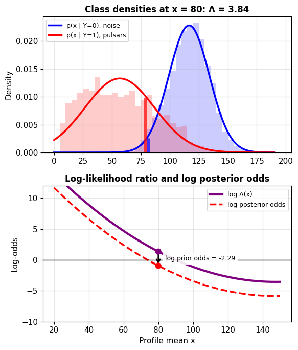
Log form: \(\log\) posterior odds \(= \log \Lambda(\mathbf{x}) + \log\) prior odds
- \(\log \Lambda(\mathbf{x})\) is the change from prior to posterior log-odds
- Independent observations: their \(\log \Lambda\) values add
Example at \(x = 80\), fitted densities:
- \(\Lambda = 0.00983 / 0.00256 = 3.84\)
- Posterior odds \(= 3.84 \times 1/9.9 = 0.39\), \(\pi = 0.28\)
- \(\Lambda > 1\): \(x\) is more probable under the pulsar class
- \(\pi < 1/2\): noise remains the more probable class
The Bayes Rule Thresholds the Likelihood Ratio
Decide pulsar when posterior odds \(> c_{01}/c_{10}\)
Substituting posterior odds \(= \Lambda(\mathbf{x}) \times\) prior odds:
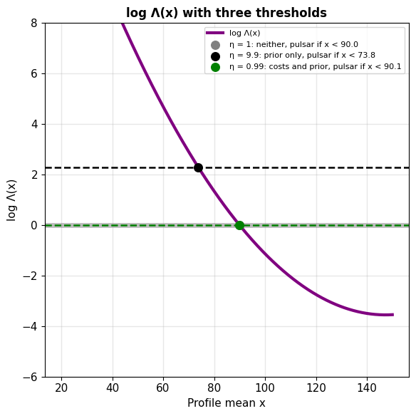
\[\Lambda(\mathbf{x}) \;>\; \eta = \frac{c_{01}}{c_{10}} \cdot \frac{P(Y=0)}{P(Y=1)}\]
- \(\Lambda(\mathbf{x})\) depends on the data only
- \(\eta\) depends on the costs and the prior only
Example: \(\eta = \dfrac{1}{10} \cdot \dfrac{16{,}259}{1{,}639} = 0.99\)
| \(\eta\) from | \(\eta\) | Pulsar if |
|---|---|---|
| Neither (equal costs, equal priors) | 1 | \(x < 90.0\) |
| Prior only | 9.9 | \(x < 73.8\) |
| Costs and prior | 0.99 | \(x < 90.1\) |
- Prior factor \(P(Y{=}0)/P(Y{=}1) = 9.9\)
- Cost factor \(c_{01}/c_{10} = 1/10\)
- For the pulsar data the two nearly cancel
With a Reject Option, the Bayes Rule Has Up to Two Thresholds
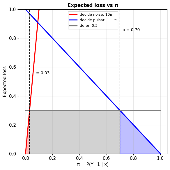
Reject option: a third action, defer the decision to a human reviewer, at cost \(c_r\)
Expected loss of each action:
- Decide noise: \(c_{10}\,\pi\)
- Decide pulsar: \(c_{01}(1-\pi)\)
- Defer: \(c_r\), for every \(\pi\)
Bayes rule, the smallest of the three:
- Noise: \(\pi < c_r / c_{10}\)
- Pulsar: \(\pi > 1 - c_r / c_{01}\)
- Defer: in between
Two thresholds only if \(c_r < \dfrac{c_{01}\,c_{10}}{c_{01} + c_{10}}\), otherwise a single threshold, \(\tau^*\)
Example, \(c_{01} = 1\), \(c_{10} = 10\), \(c_r = 0.3 < 10/11 = 0.91\), two thresholds:
- Noise: \(\pi < 0.03\)
- Pulsar: \(\pi > 0.70\)
- Defer: \(0.03 \le \pi \le 0.70\)
Equal-Variance Gaussian Classes Have Linear Log-Odds
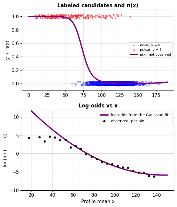
Gaussian fits to the pulsar data (spreads 17.5 and 30.0): log-odds \(= \log \Lambda(x) +\) log prior odds
\[\log \frac{\pi(x)}{1 - \pi(x)} = 0.0011\,x^2 - 0.32\,x + 17.6\]
- Quadratic in \(x\), not linear
General: classes \(\mathcal{N}(\boldsymbol{\mu}_k, \boldsymbol{\Sigma}_k)\)
Shared \(\boldsymbol{\Sigma}\): the quadratic terms cancel
\[\log \frac{P(Y=1 \mid \mathbf{x})}{P(Y=0 \mid \mathbf{x})} = \mathbf{w}^T\mathbf{x} + b, \qquad \mathbf{w} = \boldsymbol{\Sigma}^{-1}(\boldsymbol{\mu}_1 - \boldsymbol{\mu}_0)\]
\[\pi(\mathbf{x}) = \frac{1}{1 + e^{-(\mathbf{w}^T\mathbf{x} + b)}}\]
Different variances, one feature: a quadratic term remains
\[\log \frac{\pi(x)}{1 - \pi(x)} = a\,x^2 + w\,x + b, \qquad a = \frac{1}{2\sigma_0^2} - \frac{1}{2\sigma_1^2}\]
- Linear in the features \((x, x^2)\)
Data: labeled pairs \((\mathbf{x}_i, y_i)\), not densities and not \(\pi(\mathbf{x})\)
Estimating \(\pi(\mathbf{x})\) from labeled pairs:
- Estimate \(p(\mathbf{x} \mid Y=k)\) and \(P(Y=k)\), then apply Bayes theorem
- Fit \(\mathbf{w}\) and \(b\) in \(\pi(\mathbf{x}) = 1/(1 + e^{-(\mathbf{w}^T\mathbf{x} + b)})\): logistic regression
A Line Is the Wrong Shape to Model \(P(Y = 1 \mid x)\)
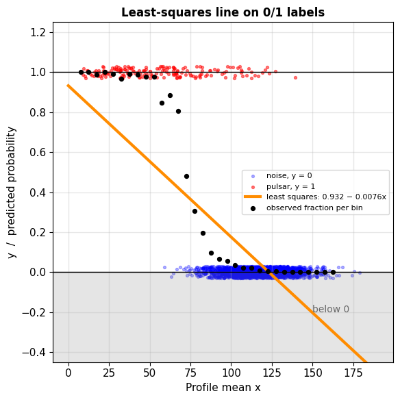
Least squares on 0/1 labels estimates \(\mathbb{E}[Y \mid X = x] = P(Y = 1 \mid x)\)
- The right quantity: the MMSE predictor
Linear model \(\hat\pi(x) = w\,x + b\):
- No bounds: below 0 at one end, above 1 at the other
- One slope: it cannot be flat in the tails and steep in between
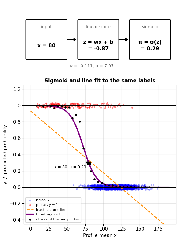
Example: least-squares line through the 17,898 pulsar labels
- \(\hat\pi(x) = 0.932 - 0.0076\,x\)
- Negative for \(x > 123\), a third of the candidates
- 0.78 at \(x = 20\), where the observed pulsar fraction is 1.00
The Log-Odds Is Unbounded
Odds \(\dfrac{\pi}{1 - \pi}\): from 0 to \(\infty\)
- \(\pi = 0.5\): odds 1 (1:1)
- \(\pi = 0.75\): odds 3 (3:1)
- \(\pi = 0.25\): odds 1/3 (1:3)
Log-odds \(\log \dfrac{\pi}{1 - \pi}\): any real number
- \(\pi = 0.5\): 0
- \(\pi = 0.75\): \(+1.10\), \(\pi = 0.25\): \(-1.10\)
- Each real value matches exactly one \(\pi\) in \((0, 1)\)
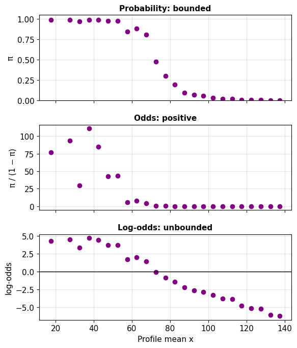
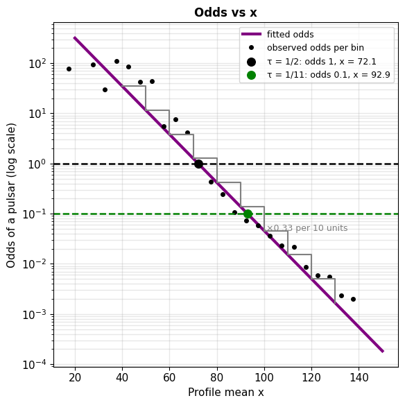
Example: observed pulsar fraction per bin of \(x\) (figure)
- Bounded on the probability scale
- Close to a line on the log-odds scale from 55 to 140
Logistic Regression Is a Linear Model for the Log-Odds
Linear score \(z = \mathbf{w}^T\mathbf{x} + b\), which can be any real number
Model: the score is the log-odds
\[\log \frac{\pi(\mathbf{x})}{1 - \pi(\mathbf{x})} = \mathbf{w}^T\mathbf{x} + b\]
Inverting: odds \(= e^{z}\), so \(\pi = e^{z}/(1 + e^{z})\)
\[\boxed{\pi(\mathbf{x}) = \sigma(\mathbf{w}^T\mathbf{x} + b), \qquad \sigma(z) = \frac{1}{1 + e^{-z}}}\]
Sigmoid:
- Between 0 and 1 for every \(z\)
- \(\pi = 1/2\) at \(z = 0\)
- Flat in both tails, steepest at \(z = 0\)
Not least squares on log-odds: a label’s log-odds is \(\log(1/0)\) or \(\log(0/1)\)
- \(\mathbf{w}\) and \(b\) come from maximum likelihood
Example, fitted to the pulsar data: \(w = -0.111\), \(b = 7.97\)
- \(x = 80\): \(z = -0.87\), \(\pi = 0.29\)
- Steepest at \(x = 72.1\), slope \(-0.028\) per unit
- Least-squares line: slope \(-0.0076\) everywhere
Poisson and Binary Classes Also Have Linear Log-Odds
Log-odds \(= \log \Lambda(\mathbf{x}) + \log\) prior odds
- Linear in \(\mathbf{x}\) whenever \(\log \Lambda(\mathbf{x})\) is linear
\(\log \Lambda\) linear in \(\mathbf{x}\):
- Gaussian classes, shared covariance
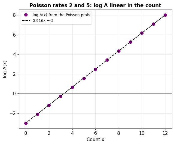
- Poisson counts, rates \(\lambda_0, \lambda_1\): \(\log \Lambda = x \log \frac{\lambda_1}{\lambda_0} - (\lambda_1 - \lambda_0)\)
- Independent binary features, \(P(x_j = 1 \mid Y = k) = \theta_{kj}\):
\[\log \Lambda = \sum_j \Big[x_j \log \frac{\theta_{1j}}{\theta_{0j}} + (1 - x_j) \log \frac{1 - \theta_{1j}}{1 - \theta_{0j}}\Big]\]
Word counts, as in spam filtering: independent Poisson counts per word give \(\log \Lambda\) linear in the count vector
- Logistic regression on counts has the form these class models imply
Other Maps from Score to Probability Fit Similar Curves
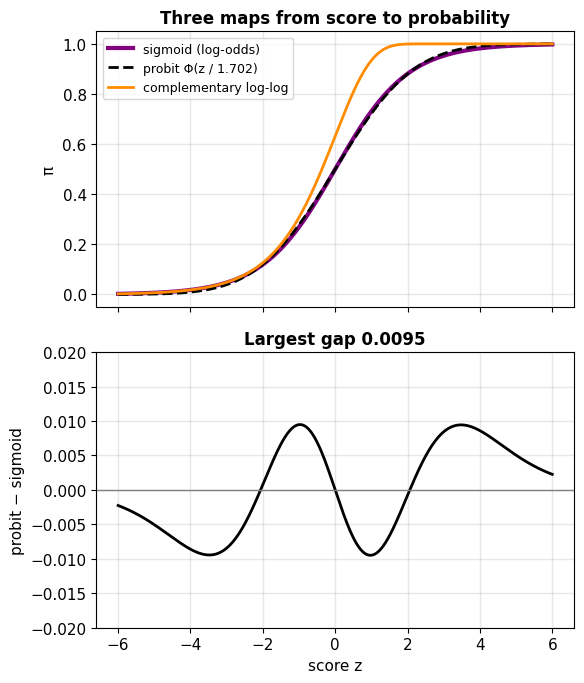
Two alternatives to the sigmoid:
- Probit: \(\pi = \Phi(\mathbf{w}^T\mathbf{x} + b)\), the Gaussian CDF
- Complementary log-log: \(\pi = 1 - \exp(-e^{\mathbf{w}^T\mathbf{x} + b})\)
Fit: nearly the same
- Probit, rescaled, stays within 0.0095 of the sigmoid
- Complementary log-log: asymmetric, approaching 1 faster than 0
Log-odds only:
- Evidence and prior add: log-odds \(= \log \Lambda(\mathbf{x}) + \log\) prior odds
- \(e^{w_j}\): the factor on the odds per unit of \(x_j\)
- Probit and log-log scores have no such reading
Reason for the sigmoid: this reading, not its fit
A One-Unit Increase in \(x_j\) Multiplies the Odds by \(e^{w_j}\)
Log-odds \(= \sum_j w_j x_j + b\)
- \(w_j\): change in log-odds when \(x_j\) rises by 1, others fixed
- \(e^{w_j}\): the factor on the odds for that increase
- \(b\): log-odds at \(\mathbf{x} = \mathbf{0}\)
Example, pulsar fit \(w = -0.111\):
- Each unit of \(x\) multiplies the odds of a pulsar by \(e^{-0.111} = 0.90\)
- Each 10 units: by \(e^{-1.11} = 0.33\)
Decision boundary \(\pi(\mathbf{x}) = \tau\): \(\;\mathbf{w}^T\mathbf{x} + b = \log \frac{\tau}{1 - \tau}\)
- A hyperplane in \(\mathbf{x}\)
- A different \(\tau\) gives a parallel hyperplane: same \(\mathbf{w}\), shifted
- Example: \(\tau = 1/2\) at \(x = 72.1\), \(\tau = 1/11\) at \(x = 92.9\)
The Sigmoid Is a Differentiable Threshold
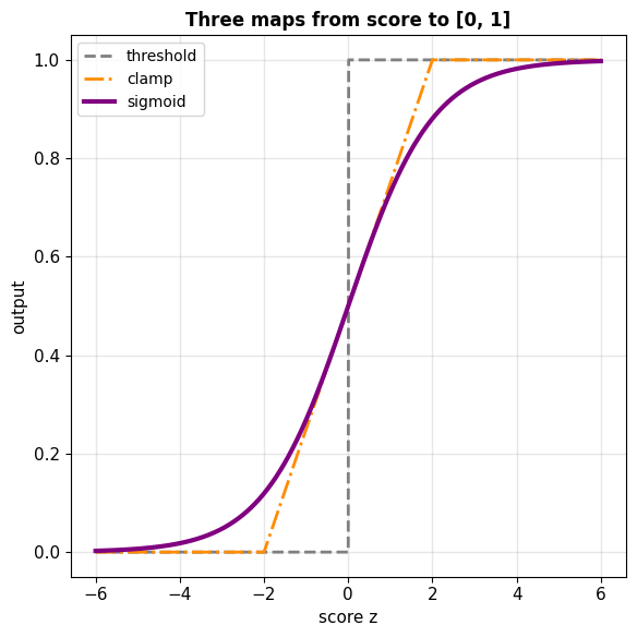
Hard threshold on the score: decide 1 if \(z > 0\)
- The Bayes rule at \(\tau = 1/2\), written on the log-odds
- Output 0 or 1, slope 0 everywhere except the jump at \(z = 0\)
Clamp \(0.5 + z/4\), cut to \([0, 1]\)
- Slope 0 outside \(|z| < 2\)
Sigmoid \(\sigma(z)\): rises from 0 to 1 around \(z = 0\)
- Output a probability, not a label
- Thresholding \(\sigma(z)\) at \(\tau\) recovers the decision
- Slope positive at every \(z\): any change in \(\mathbf{w}\) or \(b\) changes \(\pi\)
Fitting by gradient needs that slope: with the threshold or the clamp, most changes in \(\mathbf{w}\) leave the output unchanged
Sigmoid Derivative: \(\sigma' = \sigma(1 - \sigma)\)
Chain rule on \(\sigma(z) = (1 + e^{-z})^{-1}\):
\[\sigma'(z) = \frac{e^{-z}}{(1 + e^{-z})^2} = \underbrace{\frac{1}{1 + e^{-z}}}_{\sigma(z)} \cdot \underbrace{\frac{e^{-z}}{1 + e^{-z}}}_{1 - \sigma(z)}\]
\[\boxed{\sigma'(z) = \sigma(z)\,(1 - \sigma(z))}\]
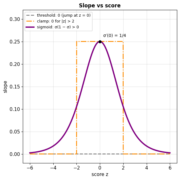
- Computed from \(\sigma(z)\) alone
- Largest at \(z = 0\): \(\sigma'(0) = 1/4\)
- Near 0 for large \(|z|\)
Example: the slope of \(\pi(x)\) is \(w\,\pi(1 - \pi)\), largest in size at \(x = 72.1\), where it is \(-0.111 \times 1/4 = -0.028\)
Negative Log-Likelihood = Summed Cross-Entropy
Each label is a Bernoulli draw given its input:
\[P(y_i \mid \mathbf{x}_i) = \pi_i^{\,y_i}(1 - \pi_i)^{1 - y_i}, \qquad \pi_i = \sigma(\mathbf{w}^T\mathbf{x}_i + b)\]
- \(y_i = 1\): \(\pi_i\)
- \(y_i = 0\): \(1 - \pi_i\)
Independent labels: the likelihood is a product
\[L(\mathbf{w}, b) = \prod_{i=1}^n \pi_i^{\,y_i}(1 - \pi_i)^{1 - y_i}\]
Negative log: the product becomes a sum
\[\mathcal{L}(\mathbf{w}, b) = -\sum_{i=1}^n \big[\,y_i \log \pi_i + (1 - y_i) \log(1 - \pi_i)\,\big]\]
- Each term: the binary cross-entropy of one label
- Maximizing \(L\) is the same as minimizing \(\mathcal{L}\)
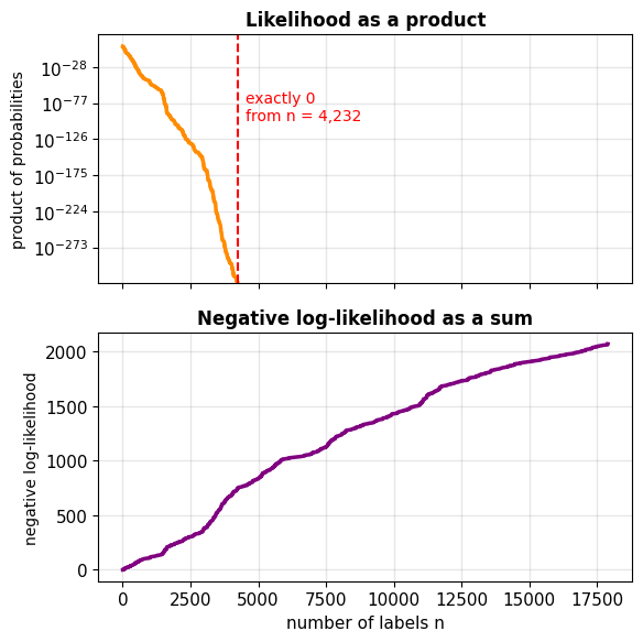
In floating point, the product underflows to 0 and the sum does not
- Pulsar labels under the fitted model: the product is exactly 0 from \(n = 4{,}232\)
Confident Wrong Predictions Dominate the Loss
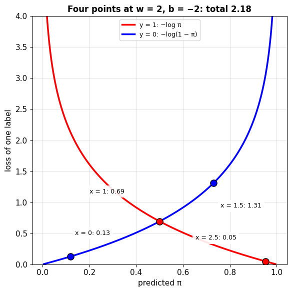
Example: four labeled points \((x_i, y_i)\)
- \((0, 0)\), \((1, 1)\), \((1.5, 0)\), \((2.5, 1)\)
- Overlap: \(y = 1\) at \(x = 1\), \(y = 0\) at \(x = 1.5\)
At \(w = 2\), \(b = -2\):
| \(x_i\) | \(y_i\) | \(\pi_i\) | loss |
|---|---|---|---|
| 0 | 0 | 0.12 | 0.13 |
| 1 | 1 | 0.50 | 0.69 |
| 1.5 | 0 | 0.73 | 1.31 |
| 2.5 | 1 | 0.95 | 0.05 |
\(\mathcal{L} = 2.18\)
- The point \((1.5, 0)\), predicted at \(\pi = 0.73\), contributes 60% of the loss
- \(-\log(1 - \pi) \to \infty\) as \(\pi \to 1\): no limit on the cost of a confident mistake
Pulsar fit: the worst-predicted 1% of candidates carry 37% of \(\mathcal{L}\)
- Pulsars at \(x\) from 130 to 139, given \(\pi \approx 0.001\): loss up to 7.4 each
Cross-Entropy Gradient Is \((\pi - y)\,\mathbf{x}\)
One label: \(z = \mathbf{w}^T\mathbf{x} + b\), \(\pi = \sigma(z)\)
\[\ell = -\big[\,y \log \pi + (1 - y) \log(1 - \pi)\,\big]\]
Chain rule:
\[\frac{\partial \ell}{\partial \pi} = -\frac{y}{\pi} + \frac{1 - y}{1 - \pi} = \frac{\pi - y}{\pi(1 - \pi)}, \qquad \frac{d\pi}{dz} = \pi(1 - \pi)\]
\[\frac{\partial \ell}{\partial z} = \pi - y\]
Weights and bias:
\[\frac{\partial \ell}{\partial \mathbf{w}} = (\pi - y)\,\mathbf{x}, \qquad \frac{\partial \ell}{\partial b} = \pi - y\]
- Prediction error times input
- Confident and right: near 0
- Confident and wrong: near \(\pm\mathbf{x}\)
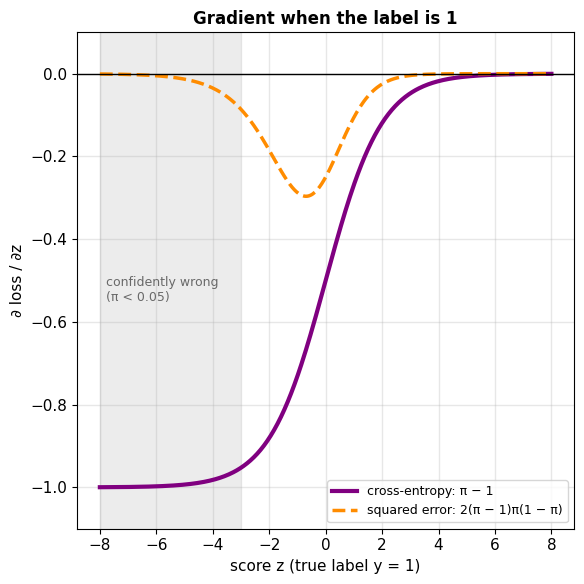
Squared error on \(\pi\) keeps the factor \(\pi(1 - \pi)\), which is near 0 when the prediction is confidently wrong (figure)
Logistic and Least-Squares Gradients Are Both \(\mathbf{X}^T(\text{prediction} - \mathbf{y})\)
Stack the data: \(\mathbf{X} \in \mathbb{R}^{n \times d}\) with rows \(\mathbf{x}_i^T\), \(\boldsymbol{\pi} = \sigma(\mathbf{X}\mathbf{w} + b\mathbf{1})\)
Sum over labels:
\[\nabla_{\mathbf{w}}\mathcal{L} = \mathbf{X}^T(\boldsymbol{\pi} - \mathbf{y}), \qquad \frac{\partial \mathcal{L}}{\partial b} = \mathbf{1}^T(\boldsymbol{\pi} - \mathbf{y})\]
Least squares, same form:
\[\nabla_{\mathbf{w}} \tfrac{1}{2}\|\mathbf{y} - \mathbf{X}\mathbf{w}\|^2 = \mathbf{X}^T(\mathbf{X}\mathbf{w} - \mathbf{y})\]
- Both: (prediction − label), weighted by the inputs
- Least squares predicts \(\mathbf{X}\mathbf{w}\); logistic predicts \(\sigma(\mathbf{X}\mathbf{w} + b\mathbf{1})\)
- Cost: \(O(nd)\) per gradient in both
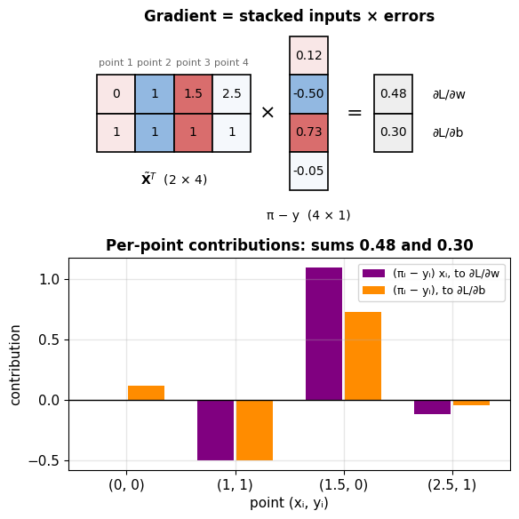
Example, four points at \(w = 2\), \(b = -2\) (figure):
- \(\partial \mathcal{L} / \partial w = 0.48 > 0\): lowering \(w\) lowers the loss
- \(\partial \mathcal{L} / \partial b = 0.30 > 0\): lowering \(b\) lowers the loss
- The point \((1.5, 0)\) contributes most of both
Logistic Regression Has No Closed-Form Solution
Stationary point:
\[\sum_{i=1}^n \big(\sigma(\mathbf{w}^T\mathbf{x}_i + b) - y_i\big)\,\mathbf{x}_i = \mathbf{0}, \qquad \sum_{i=1}^n \big(\sigma(\mathbf{w}^T\mathbf{x}_i + b) - y_i\big) = 0\]
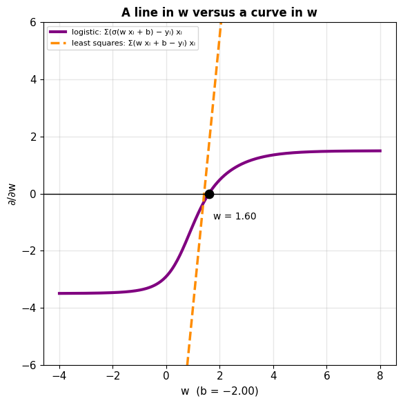
- \(\mathbf{w}\) appears inside \(\sigma\), so the equations are nonlinear in \(\mathbf{w}\)
- Least squares: \(\mathbf{X}^T\mathbf{X}\mathbf{w} = \mathbf{X}^T\mathbf{y}\) is linear and is solved in one step
- Logistic: solved by iteration
The \(b\) equation: \(\sum_i \pi_i = \sum_i y_i\)
- At the fit, the predicted number of cases equals the observed number
Example, four points: \(w = 1.60\), \(b = -2.00\)
- \(\sum_i \pi_i = 2.00 = \sum_i y_i\)
- Pulsar fit: \(\sum_i \pi_i = 1{,}639 = \sum_i y_i\)
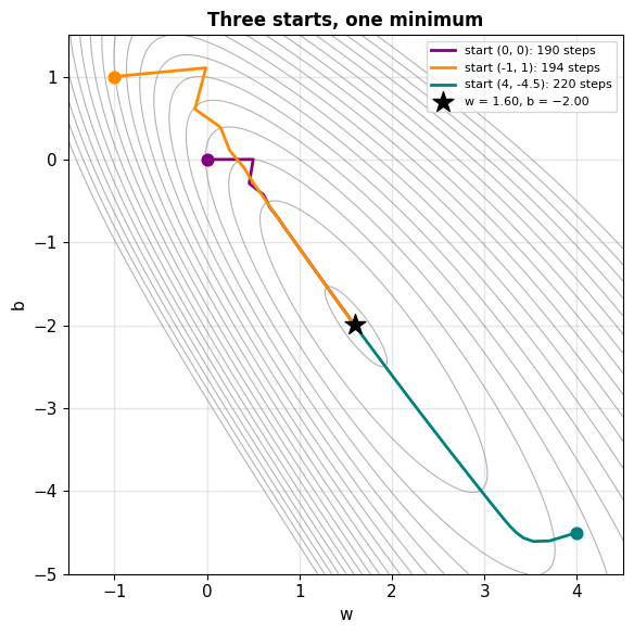
Fitted Weights Do Not Depend on the Starting Point
Zero start: \(\mathbf{w} = \mathbf{0}\), \(b = 0\)
- \(\pi = 1/2\) for every input
- \(\mathcal{L} = n \log 2\): 2.77 for the four points
Class-fraction start: \(\mathbf{w} = \mathbf{0}\), \(b = \log \dfrac{\bar y}{1 - \bar y}\)
- \(\pi = \bar y\), the fraction of class-1 labels, for every input
- Pulsar data, 9.2% pulsars: \(b = -2.29\)
- Starts closer to the answer on imbalanced data
One minimum: the loss is convex, so every start ends at the same \((\mathbf{w}, b)\)
- The start sets the number of steps, not the answer
Random starts: needed for networks, where units that start equal stay equal
Gradient Descent Repeats Predict, Differentiate, Update
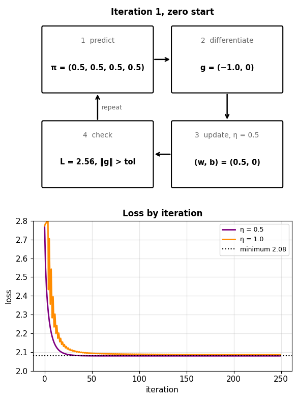
One iteration:
- Predict: \(\pi_i = \sigma(\mathbf{w}^T\mathbf{x}_i + b)\)
- Differentiate: \(\mathbf{g}_w = \mathbf{X}^T(\boldsymbol{\pi} - \mathbf{y})\), \(\;g_b = \sum_i (\pi_i - y_i)\)
- Update: \(\mathbf{w} \leftarrow \mathbf{w} - \eta\,\mathbf{g}_w\), \(\;b \leftarrow b - \eta\,g_b\)
- Stop when \(\|\mathbf{g}\|\) is small; otherwise repeat
Example, four points, zero start, \(\eta = 0.5\):
- Iteration 1: \(\mathbf{g} = (-1.0, 0)\) gives \(w = 0.5\), \(b = 0\), and \(\mathcal{L}\) falls from 2.77 to 2.56
- 190 iterations to \(\|\mathbf{g}\| < 10^{-6}\): \(w = 1.60\), \(b = -2.00\)
Step size: \(\eta < 2/\lambda_{\max}\) of the Hessian
- At the zero start: \(2 / 3.11 = 0.64\)
- \(\eta = 1\): the loss oscillates and stays above the minimum
Negative Log-Likelihood Is Convex
Hessian over \(\boldsymbol{\theta} = (\mathbf{w}, b)\), with \(\tilde{\mathbf{X}} = [\mathbf{X} \;\; \mathbf{1}]\):
\[\mathbf{H} = \tilde{\mathbf{X}}^T \mathbf{S}\, \tilde{\mathbf{X}}, \qquad \mathbf{S} = \operatorname{diag}\big(\pi_i(1 - \pi_i)\big)\]
Positive semidefinite: for any \(\mathbf{v}\)
\[\mathbf{v}^T\mathbf{H}\mathbf{v} = \sum_i \pi_i(1 - \pi_i)\,(\tilde{\mathbf{x}}_i^T\mathbf{v})^2 \ge 0\]
- Positive definite when \(\tilde{\mathbf{X}}\) has full column rank
Example at the zero start: \(\mathbf{H} = \begin{bmatrix} 2.375 & 1.25 \\ 1.25 & 1 \end{bmatrix}\), eigenvalues 3.11 and 0.26
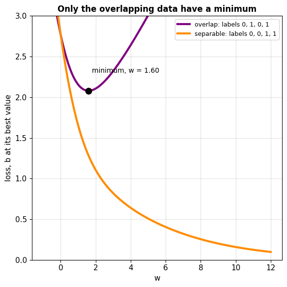
A minimum exists only if no hyperplane separates the classes
- Separable: \(\mathcal{L} \to 0\) as \(\|\mathbf{w}\| \to \infty\), a value never reached
- Pulsar subsamples of \(n = 50\): 33% separable or without a pulsar, so no minimum
Each Newton Step Solves a Weighted Least-Squares Problem
Newton: \(\boldsymbol{\theta} \leftarrow \boldsymbol{\theta} - \mathbf{H}^{-1}\mathbf{g}\), with \(\mathbf{g} = \tilde{\mathbf{X}}^T(\boldsymbol{\pi} - \mathbf{y})\), \(\mathbf{H} = \tilde{\mathbf{X}}^T\mathbf{S}\tilde{\mathbf{X}}\)
Rearranged:
\[\tilde{\mathbf{X}}^T\mathbf{S}\tilde{\mathbf{X}}\,\boldsymbol{\theta}_{\text{new}} = \tilde{\mathbf{X}}^T\mathbf{S}\,\mathbf{r}, \qquad \mathbf{r} = \tilde{\mathbf{X}}\boldsymbol{\theta} + \mathbf{S}^{-1}(\mathbf{y} - \boldsymbol{\pi})\]
- The normal equations, each point weighted by \(\pi_i(1 - \pi_i)\)
- New weights every step: iteratively reweighted least squares
Cost per step:
- Newton: \(O(nd^2)\) to form \(\mathbf{H}\), \(O(d^3)\) to solve
- Gradient descent: \(O(nd)\)
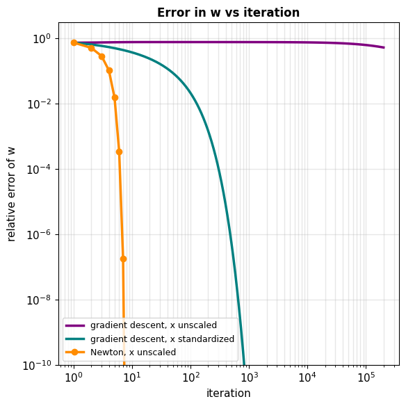
Example, pulsar data, zero start, steps to \(\hat w\) within a relative \(10^{-6}\):
- Newton, \(x\) unscaled: 7 steps
- Gradient descent, \(x\) standardized: 477 steps
- Gradient descent, \(x\) unscaled: condition number of \(\mathbf{H}\) is \(2.6 \times 10^5\)
- After 200,000 steps at the largest stable \(\eta\): \(w = -0.053\) against \(-0.111\)
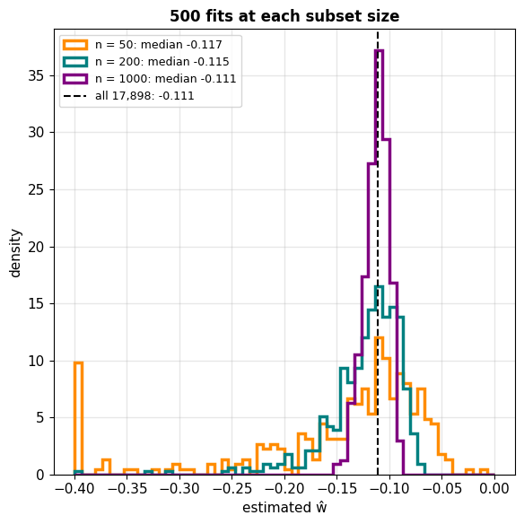
The Spread of \(\hat w\) Shrinks Roughly as \(1/\sqrt{n}\)
Reference: the fit to all 17,898 pulsar candidates, \(\hat w = -0.111\)
Subsamples: 500 random subsets at each \(n\), each fit by Newton
| \(n\) | median \(\hat w\) | middle 50% of \(\hat w\) | no finite \(\hat w\) |
|---|---|---|---|
| 50 | \(-0.117\) | \(-0.170\) to \(-0.090\) | 163 of 500 |
| 200 | \(-0.115\) | \(-0.138\) to \(-0.099\) | 1 of 500 |
| 1000 | \(-0.111\) | \(-0.120\) to \(-0.105\) | 0 |
- Spread shrinks roughly as \(1/\sqrt{n}\)
- \(n = 50\): about 5 pulsars per subset
- 33% of those subsets are separable or have no pulsar, so no finite estimate
Subsets of one data set stand in for new samples from the same survey
Gradient Descent Fits the Spam Model with the Same Loop
The loop from the four-point example, with the gradient averaged over the \(n = 4{,}000\) messages:
def sigmoid(z):
    return 1 / (1 + np.exp(-z))

n = len(y_train)
w = np.zeros(len(vocab))
b = np.log(y_train.mean() / (1 - y_train.mean()))   # class-fraction start
history = []
for step in range(1, 3001):
    p = sigmoid(X_train @ w + b)
    w -= 0.5 * X_train.T @ (p - y_train) / n
    b -= 0.5 * (p - y_train).mean()
    if step % 25 == 0:
        p_test = sigmoid(X_test @ w + b)
        history.append((step, ((p > 0.5) == y_train).mean(),
                        ((p_test > 0.5) == y_test).mean(), np.linalg.norm(w)))
Newton: a \(1{,}472 \times 1{,}472\) Hessian to form and solve at every step
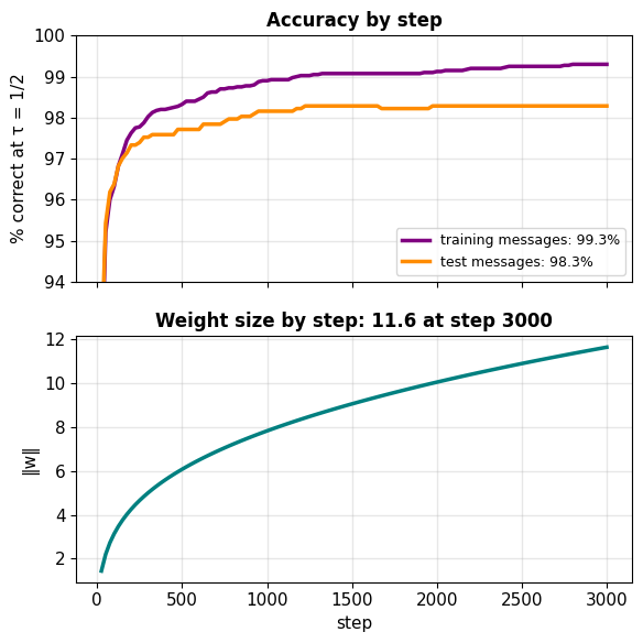
- Test accuracy: 98.3% after 3,000 steps
- \(\|\mathbf{w}\|\) still growing: the training messages are close to separable
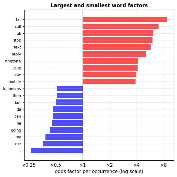
Each Word Multiplies the Odds of Spam by \(e^{w_j}\)
Odds factor \(e^{w_j}\): each occurrence of word \(j\) multiplies the odds of spam by it
Largest factors:
- “txt” 8.8, “call” 7.0, “uk” 6.2, “stop” 6.0, “text” 5.7
- Words from sign-up and reply instructions
Smallest factors:
- “i” 0.26, “me” 0.36, “my” 0.38
- First-person words, common in messages between people
Bias \(b = -4.55\): odds of spam 0.011 for a message with no vocabulary words
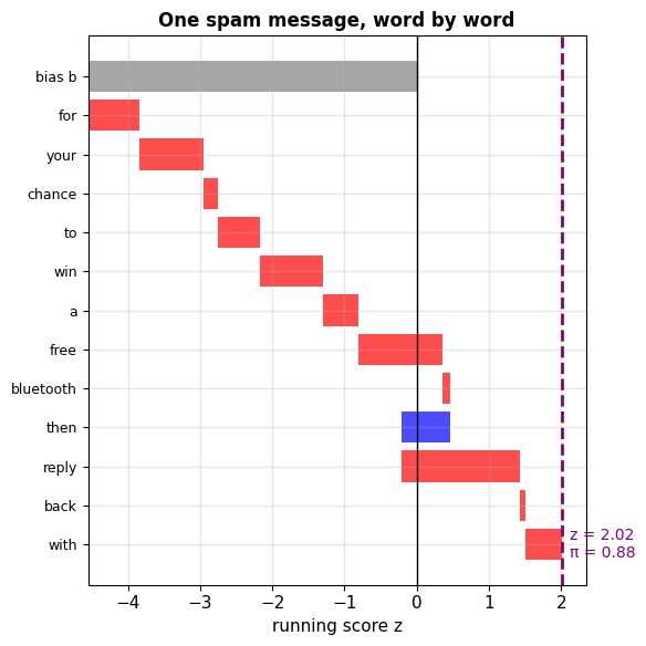
A Prediction Adds One Weight per Word
Score: \(z = b + \sum_j w_j x_j\), one term per word occurrence
Three test messages:
| Message | \(z\) | \(\pi\) |
|---|---|---|
| “For your chance to WIN a FREE Bluetooth Headset then simply reply back with “ADP”” | 2.02 | 0.88 |
| “Now am free call me pa.” | \(-1.31\) | 0.21 |
| “Latest News! Police station toilet stolen, cops have nothing to go on!” (spam) | \(-3.19\) | 0.04 |
- Legitimate message: “call” and “free” raise \(\pi\) to 0.21, still delivered
- Spam without spam vocabulary: \(\pi = 0.04\), missed
- Word counts only: no feature for meaning
\(\tau^*\) Is Optimal Only for Correct Probabilities
Threshold from the costs, \(c_{01} = 10\), \(c_{10} = 1\):
\[\tau^* = \frac{10}{10 + 1} = 0.91\]
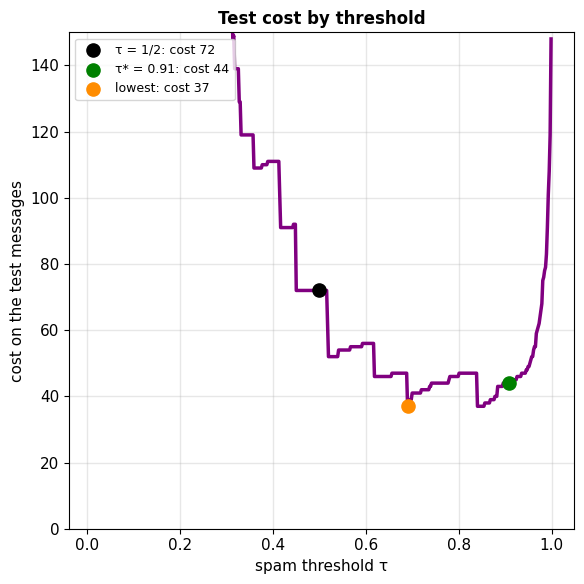
Test messages (1,574, of which 200 spam):
| Threshold | Legitimate sent to spam | Spam delivered | Cost |
|---|---|---|---|
| \(\tau = 0.5\) | 5 | 22 | 72 |
| \(\tau^* = 0.91\) | 0 | 44 | 44 |
- \(\tau^*\): 22 more spam delivered, 5 fewer legitimate messages lost
Lowest test cost: 37, at \(\tau = 0.69\), not at \(\tau^*\)
- 18 test messages have \(0.69 < \pi \le 0.91\), mean \(\pi = 0.80\)
- 17 of them are spam (94%): the fitted \(\pi\) is too low in this range
- Choosing \(\tau = 0.69\) from this curve tunes on the test set
- Threshold selection uses a validation split, not the test set
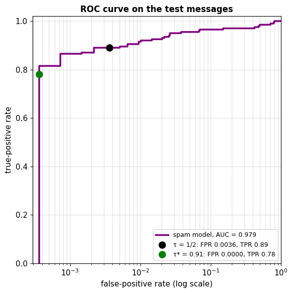
ROC Curve: Hit Rate vs False-Alarm Rate over All Thresholds
Two rates, one per true class:
\[\text{TPR} = \frac{\text{TP}}{\text{TP} + \text{FN}}, \qquad \text{FPR} = \frac{\text{FP}}{\text{FP} + \text{TN}}\]
- TPR: fraction of spam caught (recall)
- FPR: fraction of legitimate messages lost
- Each divides by one class’s size: unchanged by the spam fraction
At \(\tau = 1/2\): TPR \(= 178/200 = 0.89\), FPR \(= 5/1{,}374 = 0.0036\)
ROC curve: (FPR, TPR) as \(\tau\) runs from 1 to 0
Area under the curve (AUC): 0.979
- Probability that a random spam scores above a random legitimate message
- Depends only on the ordering of the \(\pi\) values
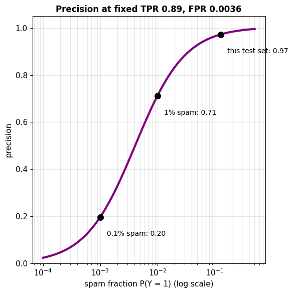
Precision Falls When the Positive Class Is Rare
Precision: fraction of messages sent to spam that are spam
\[\text{Precision} = \frac{\text{TP}}{\text{TP} + \text{FP}}\]
- At \(\tau = 1/2\): \(178/183 = 0.97\)
Same TPR and FPR, rarer spam, by Bayes theorem:
\[\text{Precision} = \frac{\text{TPR}\cdot P(Y{=}1)}{\text{TPR}\cdot P(Y{=}1) + \text{FPR}\cdot P(Y{=}0)}\]
| Spam fraction | Precision |
|---|---|
| 12.7% (this test set) | 0.97 |
| 1% | 0.71 |
| 0.1% | 0.20 |
- At 0.1% spam, legitimate messages sent to spam outnumber the spam caught 4 to 1
- The ROC curve does not change with the spam fraction
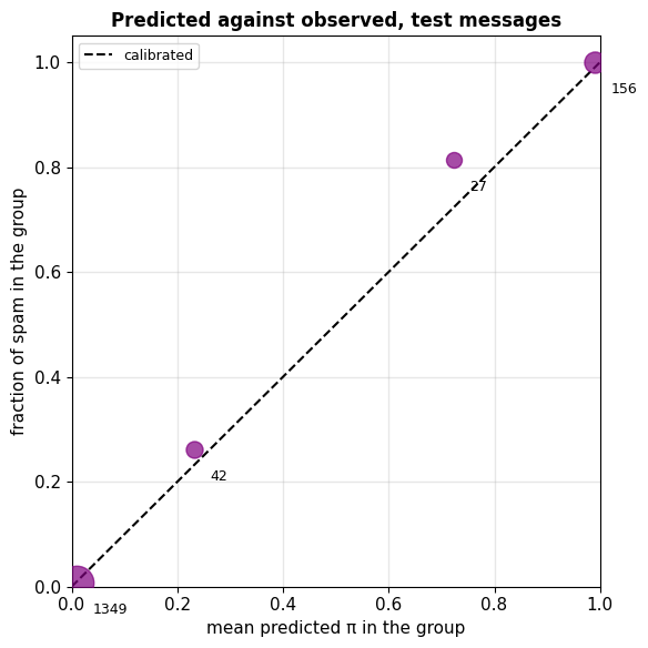
Calibration Compares \(\pi\) with the Observed Fraction of Spam
Calibrated: among messages given \(\pi \approx q\), a fraction \(q\) is spam
Test messages, grouped by \(\pi\):
| \(\pi\) range | messages | mean \(\pi\) | fraction spam |
|---|---|---|---|
| 0 to 0.1 | 1,349 | 0.009 | 0.008 |
| 0.1 to 0.5 | 42 | 0.23 | 0.26 |
| 0.5 to 0.9 | 27 | 0.72 | 0.81 |
| 0.9 to 1 | 156 | 0.99 | 1.00 |
- Close in the two outer groups, 1,505 of the 1,574 messages
- Too low from 0.5 to 0.9: mean \(\pi\) 0.72, observed 0.81
- The messages that put the lowest test cost below \(\tau^*\) are in this range
- Total: \(\sum_i \pi_i = 196\) against 200 spam
Separate from ranking: rescaling \(\pi\) without reordering changes calibration and leaves the ROC curve unchanged
Overfitting = Training Loss Keeps Falling, Test Loss Does Not
Log-loss: the negative log-likelihood per message
- Measures ranking and calibration together
- On the training messages: the quantity gradient descent minimizes
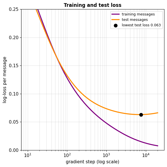
Spam model, by gradient step:
| step | training log-loss | test log-loss | \(|\mathbf{w}|\) |
|---|---|---|---|
| 300 | 0.081 | 0.094 | 5.0 |
| 3,000 | 0.027 | 0.065 | 11.6 |
| 20,000 | 0.008 | 0.066 | 22.0 |
- Training loss keeps falling as \(\|\mathbf{w}\|\) grows
- Test loss is lowest near 0.063, around step 7,000, then rises
- After step 7,000, further steps fit the training messages, not new ones
With \(K\) Classes, the Bayes Rule Compares \(K\) Expected Losses
Posterior: a vector \(\boldsymbol{\pi}(\mathbf{x}) = [\pi_1(\mathbf{x}), \ldots, \pi_K(\mathbf{x})]^T\), with \(\pi_k(\mathbf{x}) = P(Y = k \mid \mathbf{x})\)
- Nonnegative entries that sum to 1: a point on the probability simplex
Cost matrix \(\mathbf{C} \in \mathbb{R}^{K \times K}\): \(c_{ka}\) = cost of deciding \(a\) when the class is \(k\)
Expected loss of deciding \(a\):
\[R(a \mid \mathbf{x}) = \sum_{k=1}^K c_{ka}\,\pi_k(\mathbf{x}), \qquad \text{all } K \text{ at once: } \mathbf{C}^T\boldsymbol{\pi}(\mathbf{x})\]
Bayes rule: \(\delta^*(\mathbf{x}) = \arg\min_a R(a \mid \mathbf{x})\)
- 0-1 loss: \(\arg\max_k \pi_k(\mathbf{x})\), the MAP rule
- No single threshold: straight lines on the simplex separate the decisions
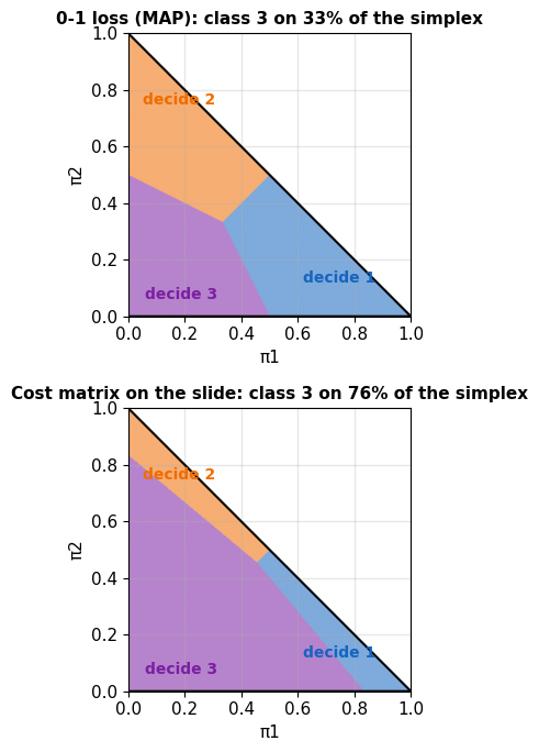
Example, \(K = 3\), class 3 costly to miss:
\[\mathbf{C} = \begin{bmatrix} 0 & 1 & 1 \\ 1 & 0 & 1 \\ 5 & 5 & 0 \end{bmatrix}\]
- Class 3 is decided on 76% of the simplex, against 33% under 0-1 loss
One-vs-Rest Probabilities Do Not Sum to 1
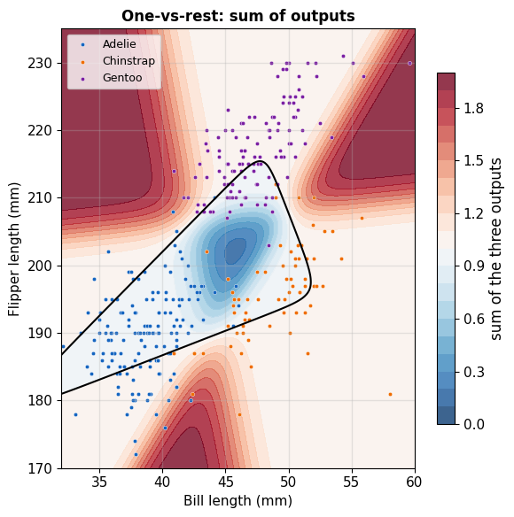
One-vs-rest: \(K\) binary logistic models, class \(k\) against the other \(K - 1\)
- Reuses the two-class model
- Each fit separately: nothing ties the \(K\) outputs together
Example data: 342 penguins, three species
- 151 Adelie, 68 Chinstrap, 123 Gentoo
- \(\mathbf{x}\) = bill length and flipper length (mm)
One-vs-rest on these birds:
- Sum of the three outputs: 0.28 to 1.97 across the birds
- 24% of the birds: sum outside 0.9 to 1.1
Argmax of the \(K\) outputs still gives a label
Expected losses \(\mathbf{C}^T\boldsymbol{\pi}\) need a probability vector
Data: Palmer Penguins, A. M. Horst, A. P. Hill, K. B. Gorman, 2020 (CC0); collected by K. Gorman and Palmer Station LTER
Softmax Maps \(K\) Scores to a Probability Vector
Softmax of scores \(\mathbf{z} \in \mathbb{R}^K\):
\[\operatorname{softmax}(\mathbf{z})_k = \frac{e^{z_k}}{\sum_{j=1}^K e^{z_j}}\]
- Exponentiating: every entry positive
- Normalizing: entries sum to 1
- Order kept: a larger score gives a larger probability
- One score far above the rest: output near one-hot
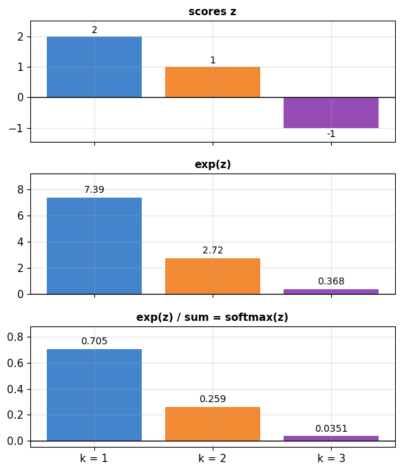
Example, \(\mathbf{z} = [2, 1, -1]\):
- \(e^{\mathbf{z}} = [7.39, 2.72, 0.37]\), sum 10.48
- \(\operatorname{softmax}(\mathbf{z}) = [0.705, 0.259, 0.035]\)
Scores tripled, \(\mathbf{z} = [6, 3, -3]\): \([0.953, 0.047, 0.0001]\)
- Larger gaps, closer to one-hot
Shared-Covariance Gaussian Classes Have Softmax Posteriors
Log of each numerator of Bayes theorem, classes \(\mathcal{N}(\boldsymbol{\mu}_k, \boldsymbol{\Sigma})\):
\[\log P(Y{=}k)\,p(\mathbf{x} \mid Y{=}k) = z_k(\mathbf{x}) \underbrace{-\,\tfrac{1}{2}\mathbf{x}^T\boldsymbol{\Sigma}^{-1}\mathbf{x} + \text{const}}_{\text{same for every } k}\]
\[z_k(\mathbf{x}) = \mathbf{w}_k^T\mathbf{x} + b_k\]
\[\mathbf{w}_k = \boldsymbol{\Sigma}^{-1}\boldsymbol{\mu}_k, \qquad b_k = -\tfrac{1}{2}\boldsymbol{\mu}_k^T\boldsymbol{\Sigma}^{-1}\boldsymbol{\mu}_k + \log P(Y{=}k)\]
Normalizing: the shared term cancels
\[\pi_k(\mathbf{x}) = \frac{e^{z_k(\mathbf{x})}}{\sum_{j=1}^K e^{z_j(\mathbf{x})}} = \operatorname{softmax}(\mathbf{z}(\mathbf{x}))_k\]
- \(K = 2\): \(\pi_2 = \sigma(z_2 - z_1)\), the two-class logistic posterior
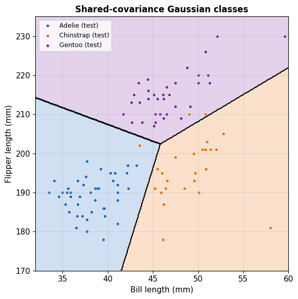
- Boundaries between classes: straight lines, \(z_k = z_j\)
Example: one Gaussian per species with a shared covariance, fit to the 240 training penguins
- 99 of the 102 test birds decided correctly
Multinomial Logistic Regression Is a Softmax of \(K\) Linear Scores
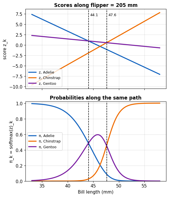
Model: one weight vector and one bias per class
\[\mathbf{z} = \mathbf{W}\mathbf{x} + \mathbf{b}, \qquad \boldsymbol{\pi}(\mathbf{x}) = \operatorname{softmax}(\mathbf{z})\]
- \(\mathbf{W} \in \mathbb{R}^{K \times d}\), row \(k\) is \(\mathbf{w}_k^T\); \(\mathbf{b} \in \mathbb{R}^K\)
- \(K(d + 1)\) parameters, fit by maximum likelihood; penguins: 9
Pairwise log-odds, linear:
\[\log \frac{\pi_k(\mathbf{x})}{\pi_j(\mathbf{x})} = (\mathbf{w}_k - \mathbf{w}_j)^T\mathbf{x} + (b_k - b_j)\]
- Each pair of classes: a two-class logistic model
- Boundary between \(k\) and \(j\): the hyperplane \(z_k = z_j\)
- Region of class \(k\): the \(K - 1\) half-spaces \(z_k > z_j\), intersected, a convex set
Assumption: every pairwise log-odds is linear in \(\mathbf{x}\); no model of \(p(\mathbf{x} \mid Y = k)\)
Example, flipper 205 mm: Adelie below a bill length of 44.1 mm, Gentoo to 47.6 mm, Chinstrap above
Softmax Cross-Entropy \(= -z_y + \log \sum_k e^{z_k}\)
One label \(y \in \{1, \ldots, K\}\), one-hot \(\mathbf{y}\): the categorical cross-entropy, the negative log-likelihood of a discrete label
\[\ell = -\sum_{k=1}^{K} y_k \log \pi_k = -\log \pi_y\]
Softmax substituted:
\[\ell = -z_y + \log \sum_{k=1}^{K} e^{z_k}\]
- Second term, the log-sum-exp: at least \(\max_k z_k\)
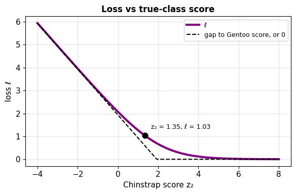
- One wrong class far ahead: \(\ell \approx z_{\max} - z_y\), linear in the gap
Data set: \(\mathcal{L}(\mathbf{W}, \mathbf{b}) = \sum_{i=1}^{n} \ell_i\)
\(K = 2\), \(z_1 = 0\), labels \(y \in \{0, 1\}\): \(\ell = \log(1 + e^{z}) - y\,z\), the binary cross-entropy
Example: a test penguin, Chinstrap, bill 50.8 mm, flipper 210 mm
| Adelie | Chinstrap | Gentoo | |
|---|---|---|---|
| \(z_k\) | \(-3.28\) | 1.35 | 1.93 |
| \(\pi_k\) | 0.003 | 0.357 | 0.640 |
- Decided Gentoo: the Gentoo score is 0.58 higher
- \(\ell = -1.35 + \log(e^{-3.28} + e^{1.35} + e^{1.93}) = 1.03 = -\log 0.357\)
Gradient Descent Fits Multinomial Logistic Regression with the Same Loop
Standardized features, averaged gradient:
W, b = np.zeros((3, 2)), np.zeros(3)
for step in range(20000):
    P = softmax(X_train @ W.T + b)       # n x K
    W -= 0.5 * (P - Y_train).T @ X_train / n
    b -= 0.5 * (P - Y_train).mean(axis=0)
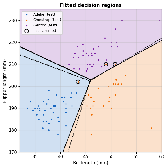
Penguins, 240 training and 102 test birds:
- Converged: gradient norm below \(10^{-9}\), training loss 0.126 per bird
- 99 of 102 test birds correct
Test confusion matrix, rows the true species:
| Adelie | Chinstrap | Gentoo | |
|---|---|---|---|
| Adelie | 43 | 0 | 0 |
| Chinstrap | 1 | 22 | 2 |
| Gentoo | 0 | 0 | 34 |
- \(K(K - 1) = 6\) kinds of error; all 3 errors are Chinstraps
The Likelihood Has No Maximum on Separable Data
Separable: a hyperplane (in one dimension, a threshold) with every training point on the side of its class
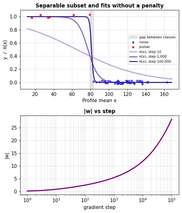
Example: 50 pulsar candidates, 6 of them pulsars
- Every pulsar: profile mean at most 79.1
- Every noise candidate: at least 83.1
Sharper threshold, lower loss: multiplying \(\mathbf{w}\) and \(b\) by \(c > 1\) keeps the boundary and steepens \(\pi(x)\)
- Every point’s loss decreases
- \(\mathcal{L} \to 0\) as \(\|\mathbf{w}\| \to \infty\): no finite minimizer
- In the limit, \(\pi(x)\) is a step: 0 or 1 at every training point
- Gradient descent: \(|w|\) = 0.8, 5.4, 28.3 after 10, 1,000, 100,000 steps
Spam training messages: close to separable, \(\|\mathbf{w}\| = 22.0\) at step 20,000 and still growing
With an L2 Penalty, the Minimizer Is Unique and Finite
Penalized loss, bias not penalized:
\[R_\lambda(\mathbf{w}, b) = \frac{1}{n}\mathcal{L}(\mathbf{w}, b) + \frac{\lambda}{2}\|\mathbf{w}\|^2\]
- Same penalty as ridge regression
Unique: Hessian \(\frac{1}{n}\tilde{\mathbf{X}}^T\mathbf{S}\tilde{\mathbf{X}} + \lambda\,\operatorname{diag}(1, \ldots, 1, 0)\) is positive definite
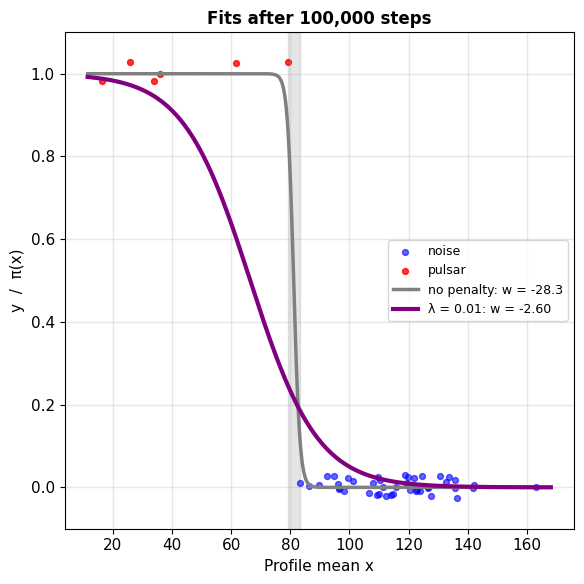
Finite: \(R_\lambda \to \infty\) as \(\|\mathbf{w}\| \to \infty\), also for separable data
Gradient step:
\[\mathbf{w} \leftarrow (1 - \eta\lambda)\,\mathbf{w} - \frac{\eta}{n}\mathbf{X}^T(\boldsymbol{\pi} - \mathbf{y})\]
- Factor \(1 - \eta\lambda\) on \(\mathbf{w}\) every step: weight decay
Example, the separable subset, \(\lambda = 0.01\): \(w = -2.60\) at step 1,000 and at step 100,000
L2 and L1 Penalties Correspond to Gaussian and Laplace Priors
MAP estimate:
\[\hat{\mathbf{w}}_{\text{MAP}} = \arg\min_{\mathbf{w}, b}\; \mathcal{L}(\mathbf{w}, b) - \log p(\mathbf{w})\]
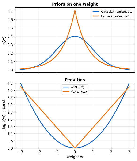
Gaussian prior, independent \(w_j \sim \mathcal{N}(0, \tau^2)\):
\[-\log p(\mathbf{w}) = \frac{\|\mathbf{w}\|^2}{2\tau^2} + \text{const}\]
- L2 penalty, \(\lambda = 1/(n\tau^2)\)
- Ridge regression: \(\lambda = \sigma^2/(n\tau^2)\), \(\sigma^2\) the noise variance
Laplace prior, independent \(p(w_j) = \frac{1}{2s}e^{-|w_j|/s}\):
\[-\log p(\mathbf{w}) = \frac{\|\mathbf{w}\|_1}{s} + \text{const}\]
- L1 penalty \(\lambda_1\|\mathbf{w}\|_1\), \(\lambda_1 = 1/(ns)\)
Narrower prior: larger penalty
The L1 Solution Has Exact Zeros, the L2 Solution Does Not
One weight, loss \(\tfrac{1}{2}(w - a)^2\) around the unpenalized value \(a\):
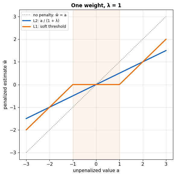
| Penalty | \(\hat w\) | \(\hat w = 0\) when |
|---|---|---|
| \(\tfrac{\lambda}{2}w^2\) | \(\dfrac{a}{1 + \lambda}\) | \(a = 0\) |
| \(\lambda \lvert w \rvert\) | \(\operatorname{sign}(a)\max(\lvert a \rvert - \lambda,\, 0)\) | \(\lvert a \rvert \le \lambda\) |
Penalty slope at \(w = 0\):
- L2: \(\lambda w = 0\), so any nonzero loss slope moves \(\hat w\) off 0
- L1: \(\pm\lambda\), so a loss slope smaller than \(\lambda\) leaves \(\hat w\) at 0
Many weights: \(\hat w_j = 0\) whenever \(\lvert \partial(\text{loss}) / \partial w_j \rvert \le \lambda\) at the solution
With an L1 Penalty, Most Spam Word Weights Are Exactly Zero
Proximal gradient: a gradient step, then the soft threshold on every weight
def soft(v, t):
    return np.sign(v) * np.maximum(np.abs(v) - t, 0)

p = sigmoid(X_train @ w + b)
w = soft(w - eta * X_train.T @ (p - y_train) / n, eta * lam)
Spam model, 5,000 steps:
| \(\lambda\) | words kept | test accuracy | test log-loss |
|---|---|---|---|
| 0 | 1,471 | 98.3% | 0.065 |
| \(3 \times 10^{-4}\) | 194 | 97.9% | 0.076 |
| \(10^{-3}\) | 85 | 97.1% | 0.097 |
| \(3 \times 10^{-3}\) | 38 | 96.0% | 0.132 |
- Positive at \(\lambda = 3 \times 10^{-3}\): “txt”, “call”, “uk”, “stop”, “text”
- Negative: “i”, “me”, “my”
Subgradient steps, \(\lambda\operatorname{sign}(\mathbf{w})\) added to the gradient: no weight exactly 0 after 5,000 steps
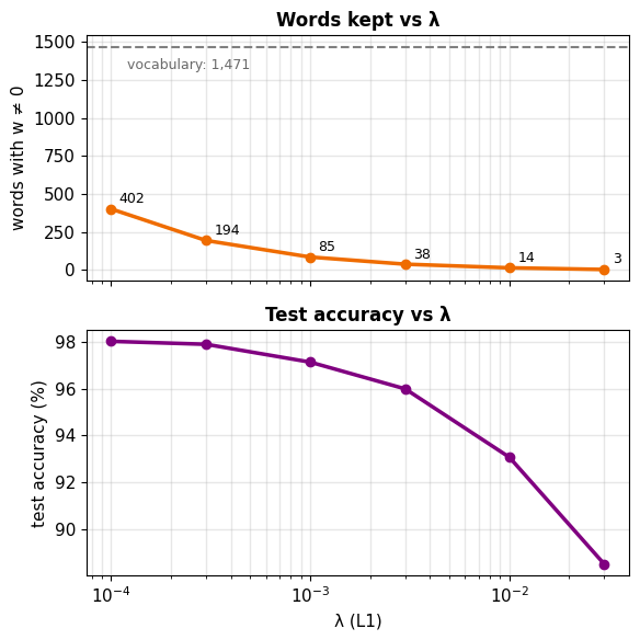
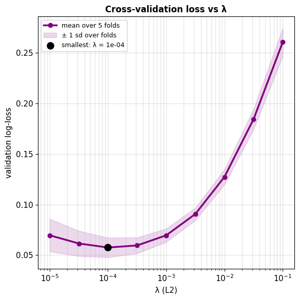
Cross-Validation Compares Values of \(\lambda\) Using Only Training Data
5-fold cross-validation on the 4,000 training messages:
- For each \(\lambda\): fit on 4 of 5 parts, log-loss on the fifth
- Average over the 5 choices of held-out part
- Cost: 5 fits per \(\lambda\), 45 fits for 9 values
Spam model, L2: lowest average log-loss 0.058, at \(\lambda = 10^{-4}\)
- Refit on all 4,000, then one test evaluation
- Test log-loss 0.063, accuracy 98.2%
- Equal to the best test loss of the unpenalized run, without using the test set
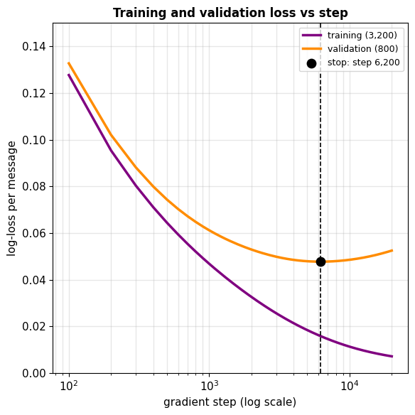
Early Stopping Ends Gradient Descent at the Lowest Validation Loss
Validation split: 800 of the 4,000 training messages; gradient descent on the other 3,200
Stopping rule: the step with the lowest validation loss
- Spam model: step 6,200, validation log-loss 0.048
- One test evaluation: log-loss 0.065, accuracy 98.2%
Relation to L2: from \(\mathbf{w} = \mathbf{0}\), \(\|\mathbf{w}\|\) grows with the number of steps
- Stopping early keeps \(\|\mathbf{w}\|\) smaller: 15.2 at step 6,200
- The step count is tuned in place of \(\lambda\)
- One run, no refits, 800 fewer training messages
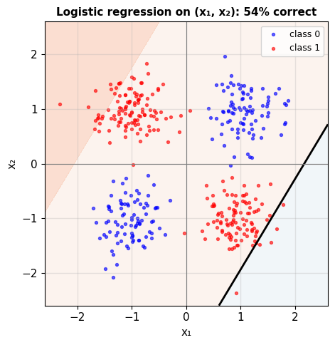
The XOR Problem: No Hyperplane Separates the Two Classes
XOR: class 1 where \(x_1\) and \(x_2\) have opposite signs
- The two class-1 quadrants lie on a diagonal
- A hyperplane splits the plane into two half-planes
- No line puts both class-1 quadrants on one side: any line misclassifies at least one quadrant
Logistic fit on 400 points:
- Weights near 0, \(\pi\) between 0.49 and 0.62 everywhere
- 54% correct
Every model in this lecture has this limit
- Logistic regression: one hyperplane
- Softmax regression: \(K\) linear scores, hyperplane boundaries
Polynomial Features Separate XOR at a Combinatorial Cost
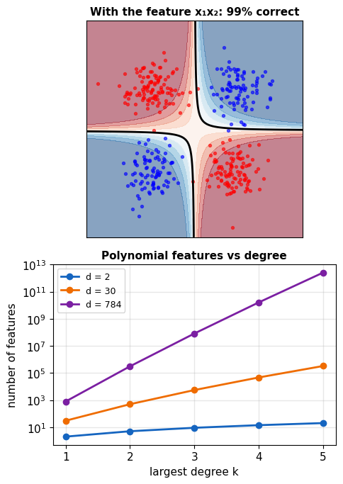
Added feature \(x_1 x_2\): logistic regression on \((x_1, x_2, x_1 x_2)\)
- A hyperplane in the three features separates the classes: 99% correct
- Still linear in the parameters, as for polynomial regression
Choosing the feature: \(x_1 x_2\) comes from knowing the pattern
- Without that knowledge: every product of inputs up to degree \(k\)
Number of features, all monomials of degree 1 to \(k\) in \(d\) inputs: \(\binom{d + k}{k} - 1\)
| \(d\) | \(k = 2\) | \(k = 3\) |
|---|---|---|
| 2 | 5 | 9 |
| 30 | 495 | 5,455 |
| 784 (\(28 \times 28\) image) | 308,504 | 80,931,144 |
Logistic Regression Is One Neuron
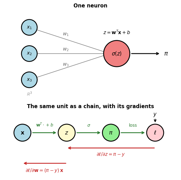
Neuron: a weighted sum plus a bias, then a nonlinearity
\[z = \mathbf{w}^T\mathbf{x} + b, \qquad a = \sigma(z)\]
- Logistic regression: one sigmoid neuron, \(a = \pi(\mathbf{x})\)
- Softmax regression: a layer of \(K\) neurons on the same input
Fitting the neuron, as in this lecture:
- Loss: cross-entropy, the negative log-likelihood
- Gradient: \(\partial \ell / \partial z = \pi - y\), \(\;\partial \ell / \partial \mathbf{w} = (\pi - y)\,\mathbf{x}\)
- Update: a gradient-descent step on \(\mathbf{w}\) and \(b\)
Label at the output: \(y\) enters the gradient through \(\pi - y\)
In a Two-Layer Network, the Features Are Fit from Data
Hidden layer: \(m\) logistic units on the input
\[\mathbf{h} = \sigma(\mathbf{W}_1\mathbf{x} + \mathbf{b}_1), \qquad \mathbf{W}_1 \in \mathbb{R}^{m \times d}\]
Output unit: logistic regression on \(\mathbf{h}\)
\[\pi = \sigma(\mathbf{w}_2^T\mathbf{h} + b_2)\]
- The features \(\mathbf{h}\) replace the hand-chosen products; \(\mathbf{W}_1\) is fit with \(\mathbf{w}_2\)
- \((d + 1)m + m + 1\) parameters: \(d = 784\), \(m = 100\) gives 78,601, against 308,504 degree-2 features
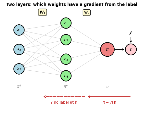
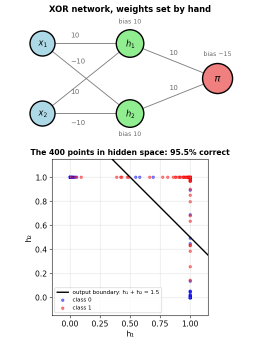
XOR with \(m = 2\), weights set by hand (figure):
- \(h_1 = \sigma(10(x_1 + x_2 + 1))\), \(\;h_2 = \sigma(10(1 - x_1 - x_2))\)
- \(\pi = \sigma(10(h_1 + h_2 - 1.5))\)
- 95.5% of the 400 points correct
- Weights not scaled by 10: \(\pi\) between 0.43 and 0.49 at every corner
The Gradient for \(\mathbf{W}_1\) Must Pass Through the Output Unit
Output weights \(\mathbf{w}_2\): logistic regression on \(\mathbf{h}\)
- Gradient \((\pi - y)\,\mathbf{h}\), with the label at the output
Hidden weights \(\mathbf{W}_1\): no label at \(\mathbf{h}\), so no \(\pi - y\) there
- A change in \(\mathbf{W}_1\) changes \(\mathbf{h}\), then the score \(\mathbf{w}_2^T\mathbf{h} + b_2\), then \(\pi\), then \(\ell\)
- The factors along that path: \(\pi - y\), the weights \(\mathbf{w}_2\), and \(\sigma' = \sigma(1 - \sigma)\)
Cost of the hidden layer:
- Loss not convex in \(\mathbf{W}_1\): several minima, and the start matters
- All-zero start: every hidden unit has the same output and gradient, and they stay identical